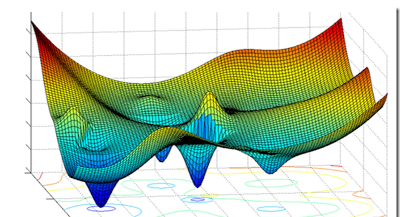
Gravitas of Gradient Descent

What is Gradient Descent?

In machine learning, an optimization algorithm is a methodical process used to modify a machine learning model's parameters in order to minimize or maximize a certain objective function(a.k.a cost function). The objective function is a mathematical depiction of the model's success or failure at a certain job. Finding the ideal collection of parameters that results in the best model performance in terms of the objective function is the aim of an optimization procedure.

Due to the fact that they allow for the training of machine learning models, optimization algorithms are essential. Gradient Descent is one such optimization algorithm and the most revered one in both Machine Learning as well as in Deep Learning. The gradient descent with the cost function in it, gauges the model’s accuracy with each iteration of parameter update until the function yields zero or almost nearing zero resulting in minimum error.

What is Gradient?

Gradient also known as the slope in mathematical terms shows how the output changes with small changes in the input. With respect to machine learning,

y: Output of the cost function

x: Trainable parameters (weights and biases)

How does Gradient Descent works?

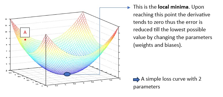
Upon initialisation of the weights we are at point A in the very beginning , where we have to decide which will be the path with the steepest descent reaching first to the local minima in the 3D plane. This required direction is the direction exactly opposite to the direction of the gradient.

Learning Rate

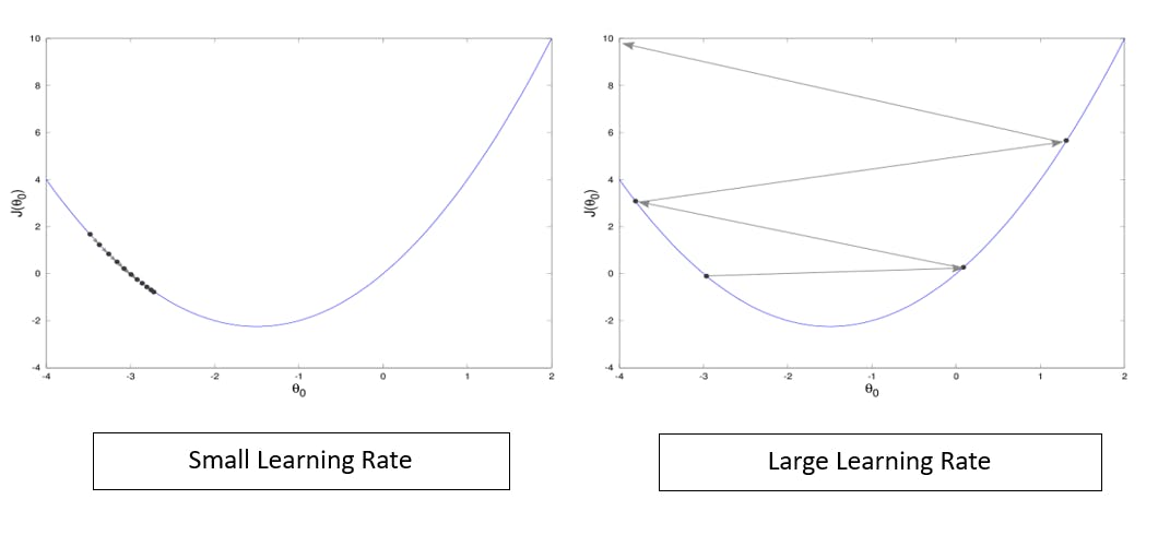
Upon selecting the direction of descent we will have to select a proper Learning Rate. It is a hyperparameter that determines the size of steps taken by the algorithm while updating the parameters and approaching the point where the gradient becomes zero or near zero(minimum error).

Small step size: The weight or parameter updates will be so slow that the algorithm won’t even converge and go near the vicinity of minima, taking an indefinite time to converge.

Large Step size: The weight or parameter updates will be so high that the point will move haphazardly resulting in overshooting and causing unstable inefficient convergence.

Basic Equations and Working

Here J is the Cost function and the Loss Function used is the Mean Squared Error(a very basic loss function). Here the cost function contains two parameters theta 1 and theta 2 both of which get updated to the result obtained from subtracting the gradient at that point  J(theta 1, theta 2) multiplied with the learning rate from the current parameter value.

This step continues till the weight or rather the parameter update becomes almost negligible, indicating that the gradient is equal to or in the vicinity of zero. Thus when the minima is reached the weights update stops giving us the values of the parameters that result in the minimum loss. The gradient indicates the amount that is to be changed in the current parameters to attain minimum error or loss (difference between the predicted result and the original value).

Common Mistake : In many cases, it is found that just after Step 1, Step 3 is performed which yields wrong values during the update of the next parameter. This is because J depends on both the parameters and both should be equally changed but when the aforementioned mistake is made the gradient for the next parameter changes as J becomes J(updated theta1, current theta2) resulting in faultiness of the algorithm.

Challenges

Gradient Descent had a successful history up to this point, but only while there were only convex functions available. Deep networks, which use many linear transformations, have since emerged, and their use has led to the emergence of extremely complicated graphs that are frequently not convex.

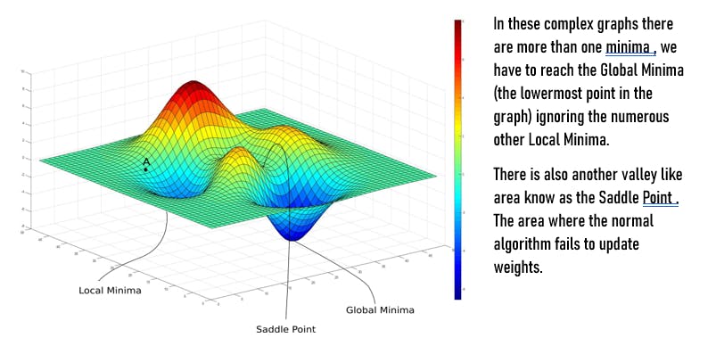
1. Local Minima : Complex deep networks build extremely complicated graphs, which in turn yield a large number of local minima. The lowest point or the global minimum cannot be obtained using the standard gradient descent process if it falls into any of these categories. We need to apply several other types of gradient descent (basically, gradient descent modified with a number of different optimization techniques) to address this issue.

2. Saddle Point : Similar to the previous example, the complicated graph, in this case, creates several valley-like areas that are parallel to the axis, nearly zero gradients, and no parameter value update, ultimately terminating the operation completely. Several other sorts of gradient descent must be used in this situation as well.

3. Vanishing & Exploding Gradient : In deep neural networks, gradients can become very small (vanishing gradients) or very large (exploding gradients) as they are propagated backward through layers. This can hinder the training process, particularly in deep architectures.

Ways to Face the Challenges

There are various ways we can improve our algorithm upon failing. We need to give place to some modification of gradient descent.

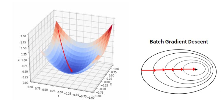
1)Batch Gradient Descent : The error for each sample in the training dataset is. calculated using batch gradient descent, commonly referred to as vanilla gradient descent. However, until every training sample has been evaluated, the model is left unchanged. Both the term "cycle" and "training epoch" are used to describe the complete process.

Batch processing has advantages such as computing efficiency, which results in a steady error gradient and stable convergence. One disadvantage is that the stable error gradient might occasionally lead to a state of convergence below the maximum that the model is capable of. Additionally, the algorithm needs access to and memory for the whole training dataset.

2) Stochastic Gradient Descent : Stochastic Gradient Descent (SGD) is a variant of Gradient Descent used to train machine learning models. Unlike traditional batch Gradient Descent, SGD computes parameter updates using small random subsets of data, making it efficient for large datasets. It converges faster due to more frequent updates and can escape local minima. However, its updates are noisy, requiring careful tuning of learning rates. Variants like mini-batch SGD strike a balance between efficiency and stability. While SGD introduces randomness and can lead to varied convergence paths, it remains a vital tool in model optimization, particularly in scenarios with limited resources or large datasets. The path retraced by the SGD is spikey as the learning rate is high .

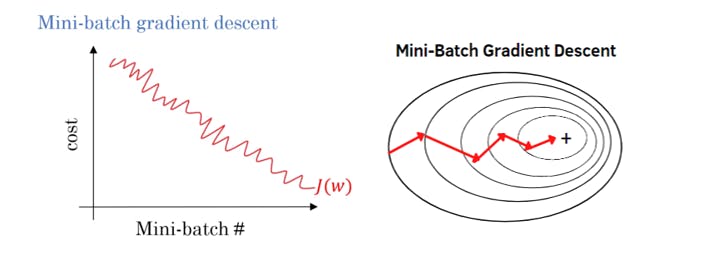
3)Mini Batch Gradient Descent : Mini-Batch Gradient Descent is a compromise .between Stochastic Gradient Descent (SGD) and batch Gradient Descent. It divides the dataset into smaller batches and computes gradient updates based on each batch. This approach combines the advantages of both SGD and batch Gradient Descent. It improves convergence speed compared to the purely stochastic updates of SGD while retaining some noise to help escape local minima. Mini-batch sizes can be adjusted to balance computational efficiency and convergence stability. This method is widely used in deep learning as it harnesses parallelism, manages memory efficiently, and strikes a practical balance between speed and accuracy during model training.

Other Techniques

There are various other techniques to modify the gradient descent algorithm according to our data, in all of them the learning rate has been used differently catering to the problems.

Some of the techniques are:-

• SGD with Momentum

• Nesterov Accelerated Gradient (NAG)

• AdaGrad optimizer

• RMSProp optimizer

• Adam optimizer

Conclusion

Throughout this post, it is very clear that Gradient Descent has been the working horse for machine learning as well as deep learning optimization. Without this, machine learning and deep learning may not hold the term precision in such high regard. The gravity of gradient descent is demonstrated here. Even if we did not go into any specifics about the better optimization described in the preceding point, considering a single post can be sufficient.